Lab 5
Introduction
The idea behind this lab is the introduction of some important analytical processes in the remote sensing field. This lab explores image mosaic, spatial and spectral image enhancement, band ratio, and binary change detection. The image mosaic part of the lab is structured to teach how to process individual scenes of satellite images to create one seamless scene. This is needed when faced with a project that covers a large geographic area that exceeds the spatial extent of one satellite image scene, or the study area astride portions of two satellite scenes.
By the end of this lab everyone will be in a position to apply all the analytical processes introduced in this lab to real life projects.
Methods
Part 1 has all to do with Image Mosaicking. Image mosaicking is done when the study area is larger than the spatial extent of one satellite image scene, or the area of interest is relatively small but traverses the portion intersected by two adjacent satellite scenes.
For the first part of this section the image eau_claire_1995p26r28.img was brought into the ERDAS viewer. But before the image could be added there were some specific functions that needed to be performed. First by clicking on the Multiple tab and then on Select Layers To Add, and then final on the Multiple Images in Virtual Mosaic button. Next click on Raster Options and click on the Select Layers To Add. In this window make sure that Background Transparent in checked along with Fit To Frame, then hit OK.
This process was then to be repeated for the second image, eau_claire_1995p25r29.img. Then both images would be brought into the same viewer, one overlapping the other.
Section 1
Finally after all this prep work Section one can really begin. Section 1 deals with Image Mosaic with the use of Mosaic Express. First click on the Raster tab to activate the tools. Then click on the Mosaic tab and then on Mosaic Express. This Process can be seen below in Figure 1.
 |
| Figure 1: This is a screenshot of the process of selecting the Mosaic Express tool. Image created by: Cyril Wilson |
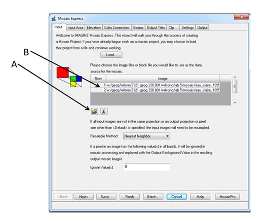
Next, in the Mosaic Express Window, click on the folder icon and add the images to be mosaicked. This process can be seen below in Figure 2.
 |
| Figure 2: This is a screenshot of the process of adding the images that are to be mosaicked. Image created by: Cyril Wilson |
Adding the eau_claire_1995p25r29.img image before the eau_claire_1995p26r29.img image will put it on top, which is what is desired for this lab. Navigate to the Output Dialog and create a folder called Mosaic_Output, this is where the image will be saved. Click on the folder next to Root Name and name the output file eau_claire1995msx.img. Then click Finish to run the model.
Section 2
This section has to deal with Image Mosaic with the use of MosaicPro. After opening the two images that were to be mosaicked before, the parameters in the Select Layers To Add tool will be the same as the section prior. First click on Mosaic and MosaicPro to open the MosaicPro window. Click on the Add Images icon. Highlight the image eau_claire_1995p25r29.img and click on the Image Area Options, then clicking on the Compute Active Area button. Click Ok. This process can be seen in Figure 3 below.
 |
| Figure 3: This is a screenshot of the process on selecting the Compute Active Area option. Image created by: Cyril Wilson |
The above steps are then repeated in adding the image eau_claire_1995p26r29.img onto the MosaicPro window.
The next task is to synchronize the radiometric properties at the area of intersection of both images so that there will be a smooth color transition from one image to the next. Click on Color Corrections, and then click on the Use Histogram Matching to activate the Set button. Select Overlap Areas, then click Ok. This process is shown below in Figure 4.
 |
| Figure 4: This is a screenshot of the above process to selecting the Overlap Areas button. Image created by: Cyril Wilson |
Initializing the image mosaic may now commence. Click on Process in the window and then Run Mosaic. Navigate to the Mosaic_Output folder and name the output image eau_claire1995msp.img.
Section 3
This section has to do with Band Ratioing. Bring in the image eau_claire_200.img. Click Raster-Unsupervised and then NDVI. The Indices interface is now open. In the input put the image eau_claire_2000.img. Name the NDVI image eau_claire2000ndvi.img. Make sure the Sensor reads "Landsat TM". Under Select Function,, make sure NDVI is highlighted. Below in Figure 5 is what the window should look like. Click Ok to create the NDVI image.
 |
| Figure 5: This is a screenshot of how the window from the above processes should look like. Image created by: Cyril Wilson |
Section 4
This next section deals with Spatial Enhancement. Bring the image Chicago_tm1995_b3.img into the ERDAS viewer. Click on Raster, Spatial, and Convolution. This will open a convolution window. This is displayed in Figure 6 below.
 |
| Figure 6: This is a screenshot of the convolution window and what it should look like. Image created by: Cyril Wilson |
Scroll down the kernel types and highlight 5x5 Low Pass. Input the image Chicago_tm1995_b3.img as the input file. Name the output file chicago_tm1995b3low.img. Then hit Ok.
Next, using the same process as above, apply a 5x5 High Pass convolution filter and name the output sierra_leone2002high.img.
The next task is going to focus on edge enhancement. Access the Convolution window and input the image sierra_leone1991.img. Under kernel type select 3x3 Laplacian Edge Detection. Check Fill under Handle Edges and uncheck Normalize The Kernel. Name the outpue sierra_leone1991edge.img and click Ok.
Section 5
This section deals with Spatial Enhancement. Bring the image eau_claire1991b3.img into the ERDAS viewer. Click on Panchromatic to activate those tools. Click on General Contrast and General Contrast again. After the Contrast Adjust interface opens click on Method and change it to Gaussian. Click apply.
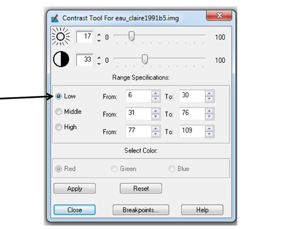
This process is going to be repeated, but except for selecting General Contrast, the Piecewise Contrast option is going to be selected. Change the values to what they are in Figure 7 below.
 |
| Figure 7: This is a screenshot of the values that are to be used for the Piecewise Contrast. Image created by: Cyril Wilson |
Next a Histogram Equalization is going to be performed. Open the image I5026029_0292011b30.img. Click on Radiometric and then Histogram Equalization. Input the above image and name the output ec_2001_b3_he.img. Then press Ok.
Section 6
This section deals with Image Differencing. The first step is to display the images ec_envs1991.img and ec_envs2001.img. Click on Functions and then click on Two Image Functions to access the Two Input Operators. Input the images above in the input file. For the output name it ec_envrns_91_11.img. Click Layer and change from All to layer 4, do the same for both images. Click Ok.
Now open the Image Metadata and click the Histogram. Estimate a point by using a rule of thumb threshold of Mean + 1.5 x Standard Deviation. Write this value down. Now put the curser over the center and write that value down. Add those two values together to find the upper limit of the change/no change threshold. Do this same procedure for the lower value.
Section 7
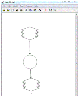
This section deals with Mapping Change Pixels in Difference Image Using Spatial Modeler. Open Model Maker by clicking on Toolbox, and Model Maker. Create a model that looks like the one in Figure 8.
 |
| Figure 8: This is a screenshot of what the model should look like for the completion of this next section. Image created by: Cyril Wilson |
For the first raster object input the image ec_envs_2001_b4.img and for the second raster object ec_envs_1991b4.img. For the function write $n1_ec_envs_2001_b4 - $n2_ec_envs_1991_b4 + 127. Name the output ec_91-11chg_b.img. Then run the model. Bring this created image into the viewer and complete the process for finding the change/no change threshold value just like what was done above. Except multiply the standard deviation by 3 this time.
Open a new Model Maker and create a model that looks like Figure 9.
 |
| Figure 9: This is a screenshot of what the next model should look like. Image created by: Cyril Wilson |
Insert image ec_91-11chg_b.img in the input raster object. Open the function object. Change to Conditional and click on Either IF OR. The function script should look like this: EITHER 1 IF ( $n1_ec_91 > change/no change threshold value ) OR 0 OTHERWISE. Label the output image ec_91-11bvis.img. run the model and bring the image into the viewer. It should look like Figure 10.
 |
| Figure 10: This is a screenshot of what the model should have created in the process above. Image created by: Cyril Wilson |
This will then be brought into ArcMap and be set over the image ec_91-11bvis.img to show the spatial distribution of this area over the last 20 years.
Results
For the results for each section I either can to upload an image or answer a question or two. I will show you my created images and answered questions for each section below.
Section 1
Q1: As
far as color transition goes, the eau_claire_1995p2529.img image seems to have
a much more rugged color transition than that of the eau_claire_1995p26r29.img
image. The second image is much smoother than the second image. Besides the
second image being a smoother color transition, the color for this image is
also much more vibrant. The color is much brighter, but I believe this makes
viewing the image more difficult.
Section 2
Q2: Using
MosaicPro, both of the images seem to have a fairly similar brightness. The
deference is in the smoothness once again. The second image is again smoother
and more difficult to interpret features. The differences between Mosaic
Express and MosaicPro are due to user input. The MosaicPro image is much more
extensive and in depth with the overall quality than that of the Mosaic Express
image. This is because MosaicPro demands extensive user input to be able to
smooth images, perform multiple radiometric synchronization processes in order
to produce a visually pleasing and spectrally seamless image. Mosaic Express
only demands the bare minimum of inputs by the user.
Section 3
Q3: In the areas of the NDVI image that are very white I
would expect to find vegetation. As stated in the notes, several ratios to help
discriminate against objects and features have been developed. One of those
would be normalized difference vegetation index (NDVI). Because the white is so
vivid and stands out I would assume that in a NDVI image that those white areas
would in fact be vegetation.
Q4: While the white area does take up a lot of the image,
there are in fact areas of medium gray or black. These are areas that lack
vegetation. In this image there are two types of areas that lack vegetation,
the first being water. The rivers in this area are black. The second would be
the residential areas on the map. These residential areas are the medium gray
color. This would be home to features such as buildings and roads.
Section 4
Q5: A high frequency image has significant changes in
brightness values over a short distance.
Q6: The 5x5 Low Pass filtered image does in fact decrease
the changes in brightness over short distance. The image looks smoother and not
as choppy at the original image. The one this I would have to say seemed to be
a disadvantage of the 5x5 image would be that the original was much easier to
see. I synched the views and zoomed in to the Chicago area. With the original
image it was much easier to view specific features. Unlike the 5x5 image where
it was blurry and features were not as distinguishable.
Q7: A low frequency image has few changes in brightness
values over a given area.
Q8: The 5x5 High Pass filter seems to increase the changes
in brightness values over a short distance. This time the original image seems
to be smoother while the 5x5 image is much more coarse and bright. I would now
say the 5x5 image looks more suitable for the use of feature identification. I
synched the views again the 5x5 image was much easier to look at to see what
the white areas of the image were. Whether they were a river or some other
feature.
Q9: A Laplacian Convolution filter approximates a second
derivative between two adjacent pixels. It also sharpens the image by locally
increasing the contrast at discontinuities. Finally it gives an image a natural
look compared with other methods.
Q10: I’m not sure if I would consider the laplacian image as
looking more “natural”. It definitely looks more rustic with its dull colors
and more visible features. The image does look sharper than the original image.
There are certain features that do look less visible in the enhanced image,
such as crevasses and features of that nature. It is also apparent that the
image was enhanced in some way, shape, or form. There is a patterned scaring
that is shown on the image.
Section 5
Q11: The histogram for this image would seem to be
near-Gausian because of its distribution and high peak. Mode = 0.
Q12: A minimum-maximum contrast stretch on this image is
appropriate because of the low contrast of the image itself. This type of
linear enhancement is also best used in Gausian or near-Gausian histograms.
Q13: The historgram for this image would seem to be
non-Gausian because of its lack of distribution. Mode = 0.
Q14: It’s appropriate to perform a piecewise contrast
stretch on this image because it is non-Gausian. This makes it perfect for a
piecewise contrast stretch.
Q15: The Piecewise image is much coarser and shows off the
features within the image better than that of the original image. I feel like
if I had to choose one of the images for feature identification I would most
certainly choose the piecewise image over the original image. The piecewise
image is just that much more defined.
Q16: I would say it is apparent that this image is not
enhanced in any way that would make feature identification more efficient. The
contrast if fairly low just by looking at the image, the short, high peak on
the histogram also tells me that the contrast on this image is fairly low.
Q17: It is immediately apparent that there is a far greater
contrast in the second image than there is in the original image. Features are
clearer and more defined. The histogram for the second image is also more
spread out which hints to an increase in contrast from that of the original
image that has a short, high peaked histogram.
Section 6
Section 7
Q18: The spatial distribution of areas that have changed
over this 20 year period are fairly clustered together. That is because these
areas are located around urban areas and near water. I believe that the reason
these areas are the ones with change is because urban areas are always
changing, mostly due to the great number of people that are located in these
areas. If you think about it a rural area with not a lot of people isn’t really
going to change that much over 20 years. But an area with lots of people is
changing constantly, with new buildings and roads and whatnot.


No comments:
Post a Comment