Spectral Signature Analysis

Lab 8

 

 

 

Introduction

 

The purpose behind this lab is to gain experience on the measurement and interpretation of spectral reflectance (signatures) of various earth surface and near surface materials captured by satellite images. The steps behind this are as follows; collect spectral signatures from remotely sensed images, graph them, and perform analysis on them to verify whether they pass the spectral separability test. The completion of this lab will enable us remote sensing students to collect and properly analyze spectral signature curves for various earth surface and near surface features for any multispectral remotely sensed image.

 

 

Methods

 

The image that will be used for this lab is a Landsat ETM+ image that covers the Eau Claire area and a section of the Cities to collect and analyze spectral signatures of various earth surfaces. I measured and plotted the spectral reflectance of twelve materials and surfaces from the image eau_claire_2000.img. These twelve features are as follows;

• Standing Water
• Moving Water
• Vegetation
• Riparian Vegetation
• Crops
• Urban Grass
• Dry Soil (uncultivated)
• Moist Soil (uncultivated)
• Rock
• Asphalt Highway
• Airport Runway
• Concrete Surface (Parking Lot)

 

To begin the lab open up ERDAS and bring in the image eau_claire_2000.img. Zoom into the Eau Claire and Chippewa County area, then locate Lake Wissota. Click Home and then Drawing. Click on the Polygon tool. These steps are shown in the figure below.

 

 

Figure 1: This is a screenshot of the above processes of locating the Polygon tool.
Image created by: Cyril Wilson

 

 

Then proceed to digitize Lake Wissota. Next plot the spectral signature that was just collected. Click on Raster, Supervised, and then Signature Editor. After the Signature Editor is open click on Create New Signatures from AOI. This will add the signature with a default value labeled Class 1. Change the name of Class 1 to Standing Water. Then click on Display Mean Plot Window to display the spectral plot of the signature that was just collected from Lake Wissota. This process can be seen below in Figure 2.

 

 

Figure 2: This is a screenshot of the above processes from adding the signature and then displaying the spectral plot of the signature.
Image created by: Cyril Wilson

 

 

Figure 3: This is an example of what the signature plot will look like. This is the signature plat for the feature Standing Water.
 

 

Collect spectral signatures for features 2 through 12 above using the same procedure for standing water. Also change the background of the Signature Mean Plot to white.

 

 

Results

 

Q1: Band 1 (Blue) (0.45 – 0.52 µm) is the band that has the highest reflectance for standing water. Band 4 (Near IR) (0.76 – 0.90 µm) is the band that has the lowest reflectance for standing water.

Q2: The highest reflectance was seen with Band 1 (Blue) because water doesn’t do a good job of absorbing blue from the visible light spectrum. This blue visible light is then reflected back into the atmosphere, and this is why water appears blue to us.

The lowest reflectance for water was with the 4^th Band (Near IR). The reason this band has a lower reflectance is because water is able to effectively absorb the Near IR band. Since a lot of it is absorbed, there is less to be reflected out into the atmosphere.

 

Q3:

Sig 2

 

 Highest reflectance = Band 1 (0.45 – 0.52 µm); Lowest reflectance = Band 6 (10.40 – 12.50 µm)

 

Sig 3

 Highest reflectance = Band 4 (0.76 – 0.90 µm); Lowest reflectance = Band 6 (10.40 – 12.50 µm)

 

Sig 4

 

Highest reflectance = Band 5 (1.55 – 1.75 µm); Lowest reflectance = Band 3 (0.63 – 0.69 µm)

Sig 5

 

Highest reflectance = Band 5 (1.55 – 1.75 µm); Lowest reflectance = Band 2 (0.52 – 0.60 µm)

 

Sig 6

 

Highest Reflectance = Band 5 (1.55 – 1.75 µm); Lowest reflectance = Band 3 (0.63 – 0.69 µm)

Sig 7

 

Highest Reflectance = Band 5 (1.55 – 1.75 µm); Lowest reflectance = Band 4 (0.76 – 0.90 µm)

 

Sig 8

 

Highest Reflectance = Band 5 (1.55 – 1.75 µm); Lowest reflectance = Band 4 (0.76 – 0.90 µm)

Sig 9

 

Highest Reflectance = Band 5 (1.55 – 1.75 µm); Lowest reflectance = Band 4 (0.76 – 0.90 µm)

 

Sig 10

 

Highest Reflectance = Band 5 (1.55 – 1.75 µm); Lowest reflectance = Band 4 (0.76 – 0.90 µm)

Sig 11

Highest Reflectance = Band 5 (1.55 – 1.75 µm); Lowest reflectance = Band 4 (0.76 – 0.90 µm)

Sig 12

 

Highest reflectance = Band 1 (0.45 – 0.52 µm); Lowest Reflectance = Band 4 (0.76 – 0.90 µm)

 Final Signature Mean Plot

 

 

Q4:

Vegetation usually shows the highest and lowest reflectance depending on the state of the vegetation. Vegetation that is healthy and green will absorb a lot of the energy that it encounters, while vegetation that is unhealthy and dying will not need that energy and reflect that back into the atmosphere. Vegetation has the most reflectance at the Band 5 level, which has a longer wavelength. Newer vegetation will have less protein cells, which in turn that crop will reflect more because the plant doesn’t need to absorb those few protein cells. Vegetation has the least amount of reflection between Bands 2 and 3. This is because these bands measure visual light, which is absorbed by the plants to grow. So in turn these bands are not reflected back into the atmosphere, but are absorbed.

Q5:

Dry and Wet soils vary the most in the visible light spectrum, Bands 1-3. Wet soils reflect better than dry soils because of the water content of the two. Moist soils will have a higher water content, and since water reflects well, moist soils will reflect more that dry soils.

Q6:

While they do vary, Standing Water and Moving Water do have a lot of similarities. This is because they are the same substance. The motion of the water doesn’t change the reflectance enough to make them dissimilar. Another that is similar is Dry Soil and Rock. This is because they have similar characteristics and have the same moisture content for the most part, and similar visual descriptions.

Two features that are very different are Riparian Vegetation and Moist Soils. Riparian vegetation seems to have way less reflectance than that of the moist soils. This would be because of the fact that vegetation absorbs a lot more energy than soil would. The only spectral band that these two variables are similar in is the 4^th Band, otherwise they are almost polar opposites.

Q7:

The visible light bands, Bands 1-3, seem to have the highest average reflectance. It doesn’t have either the highest or lowest reflectance. Which I feel would make it perfect for collecting data from a variety of different features.

 

 

 

 

 

 

 



Photogrammetry

Lab 7

 

 

 

Introduction

 

Photogrammetry is the science of making accurate measurements from aerial photographs and satellite images and in the process obtain geometrically reliable products. The goal of this lab was to develop skills in performing photogrammetric tasks on aerial photographs and satellite images. What will be keyed on in this lab is the mathematics behind the calculation of photographic scales, measurement of areas and perimeters of features, and calculating relief displacement.

 

This lab deals with the introduction of stereoscopy and performing orthorectification on satellite images. All in all this lab is really meant to put us in the position to perform diverse photogrammetric tasks.

 

 

Methods

 

 

Part 1

 

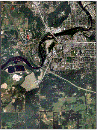
There are two tasks located in this first section. The first deals with calculating scale of nearly vertical aerial photographs. In this section we were to open up the image Eau Claire_West-se.jpg. In this image there are two points, labeled A and B. The task was to calculate the scale of this aerial photograph by using a ruler and measuring the distance on the computer screen. The only information that was given was the actual ground distance between the two points is 8822.47 ft. The image that was used for this section can be seen below in Figure 1.

 

 

Figure 1: This is the image that was used to complete section 1. The points A and B are located in the Northwestern portion of the image.
Image created by: Cyril Wilson

 

 

The second task in this section also deals with scale. Now the image ec_east-sw.img will be used. This image was taken by the National Agriculture Imagery Program (NAIP) in 2005. This aircraft acquired the photograph at an altitude of 20,000 ft. above sea level with a camera that had a focal length lens of 152 mm. One other bit of information given was that Eau Claire County is 796 ft. in elevation. The task is to use this information to figure out the scale. Looking at the image for this task isn't really necessary, it is more mathematical based.

 

 

 

 

Section 2

 

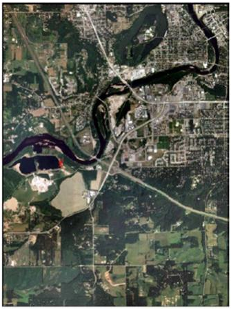
This section deals with measurement of areas of features on aerial photographs. This begins by displaying the image ec_west-se.img in an ERDAS viewer. The idea behind this section is to trace the feature located in Figure 2 and then look at the measurement window to obtain the area and perimeter of the feature.

 

 

Figure 2: This is the image that contains the feature that is to be traced for this section. The red X in the western portion of the image is the lagoon that will be measured.
Image created by: Cyril Wilson

 

 

These are the instructions as to obtaining the measurements.

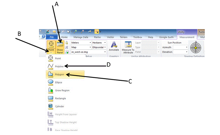
• Click the 'Measure' icon. This will change the tool panel, shown below.
• On the tool panel, click on show Panel (arrow A). This will open a View Measurements table at the bottom of the image.
• Click a Point drop down arrow (arrow B) to show various measurement tools.
• Click on the Polygon tool (arrow C) to measure the area.
• Use that tool carefully to digitize the outline of the lagoon in the photo above. The area can be read directly from the Measurement window. Click the drop down default hectares to change to other units of measuring area and perimeter.
• Click on the Polyline tool (arrow D) to measure perimeter. Follow the same process as measuring the area.

 

Figure 3: This is an image of the tools that are needed to complete this section
Image created by: Cyril Wilson

 

 

 

Section 3

 

 

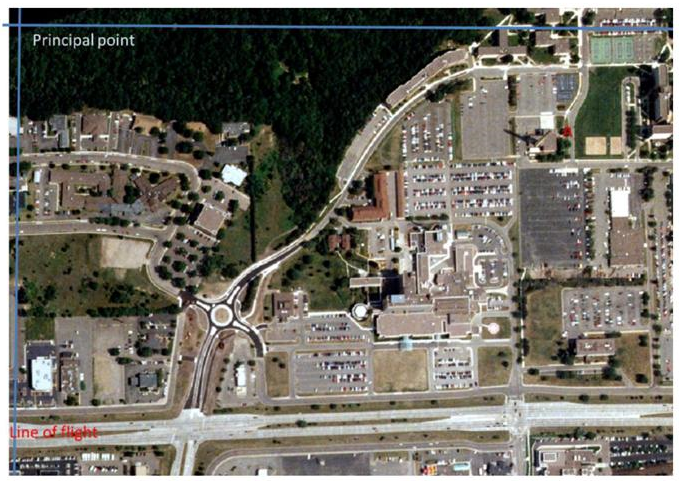
This section deals with calculating relief displacement from object height. The image used for this portion is ec_west-se.img, which can be seen below. The information given for this section is as follows; the height of the aerial camera above datum is 3,980 ft., the scale of the image is 1:3,209. Then a hint was given (hint: using a ruler to measure the height of the smoke stack and find its real world height; then measure the radial distance between the principal point and the top of the smoke stack). With data the relief displacement could then be calculated.

 

 

Figure 4: This is the image that was used to complete this section. The principal point can be seen in the top, left-hand portion of the image, while the smoke stack is marked by the red X.
Image created by: Cyril Wilson

 

 

Part 2

 

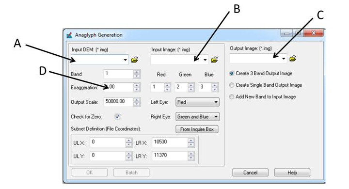
This part of the lab deals with stereoscopy. To begin, the image ec_city.img needs to be brought into a viewer in ERDAS. Then open a second viewer and bring in the image ec_dem2.img. Then click on Terrain - Anaglyph to open the Anaglyph Generation window. In the Input DEM, input ec_dem2.img. For the Input image, input ec_city.img. In the Output image, insert the image ec_anaglyph.img located in the Steroscopy_output folder. Increase the vertical exaggeration to 2. Then click OK to run the model.

 

 

Figure 5: This is the Anaglyph Generation window where the above operations are completed.
Image created by: Cyril Wilson

 

 

The final step is to use polaroid glasses to observe the image.

 

 

 

Part 3

 

This part deals with orthorectification. Erdas Imagine Lecia Photogrammetric Suite (LPS) will now be introduced. It is used in digital photogrammetry for triangulation, orthorectification of images collected by various sensors, extraction of digital surface and elevation models.

 

Tasks

• Create a new project.
• Select a horizontal reference source.
• Collect GCPs.
• Ass a second image to the block file.
• Collect GCPs in the second image.
• Perform sutomatic tie point collection.
• Triangulate the images.
• Orthorectify the images.
• View the orthoimages.
• Save the block file.

 

 

Section 1

 

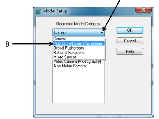
The task of creating a new project is what section 1 deals with. Open up ERDAS and open the LPS Project Manager tool. Click the Create New Block File to open the Create New Block File dialog. Then navigate to the subfolder that was created for this lab and name the block file Sat_ortho, then click OK. The Model Setup dialog is now open. This is shown below in Figure 6.

 

Figure 6: This is a screenshot of the window that was opened in the previous steps.
Image created by: Cyril Wilson

 

Click on the Geometric Model Category and choose Polynomial-based Pushbroom. In the Geometric Model Category select SPOT Pushbroom, then click OK.

 

The Block Property Setup dialog is now open. Click Set in the Horizontal Reference Coordinate System. The Projection Chooser dialog is now open. In the Custom tab click Projection Type and choose UTM. Click the Spheroid Name and select Clarke 1866. Click the Datum Name and select NAD27(CONUS). Click UTM Zone field and type 11. Then click OK. Click OK on the Block Setup dialog to close it.

 

 

Section 2

 

This section deals with adding imagery to the Block and define the sensor model. In the Block Project Tree View click the Images folder. Then click the Add Frame icon, the Image File Name dialog is now open. Add the image Spot_pan.img, then click OK.

 

Next you will verify the parameters of the SPOT pushbroom sensor. Click the Show and Edit Frame Properties icon. Click Edit, the sensor information dialog is now displayed. Click OK and then click OK again.

 

 

 

Section 3

 

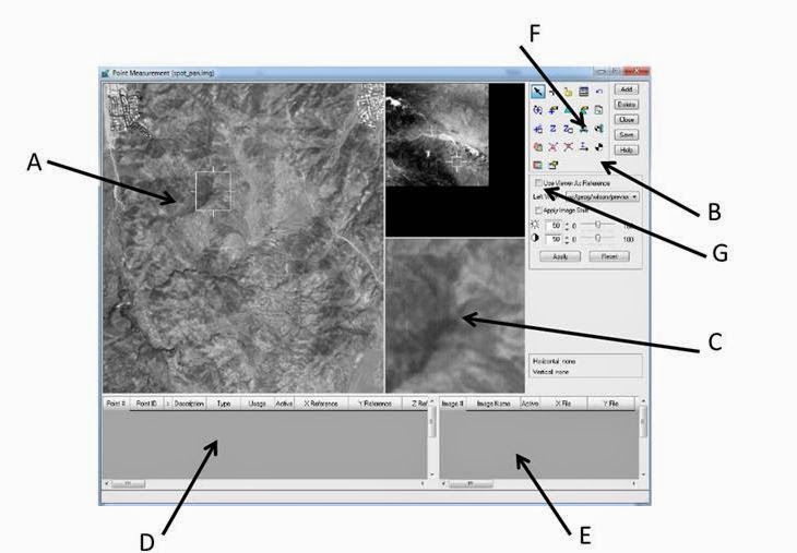
This section deals with activating the Point Measurement tool and collecting GCPs. Start by clicking the Start Point Measurement Tool and select the Classic Point Measurement Tool, then click OK. The Point Measurement tool opens displaying three views, a Main View, and two Cell Arrays.

Arrow A is the Main view, arrow B is the Tool Palette, arrow C is the Detail View, arrow D is Reference Cell Array, and arrow E is the File Cell Array. These are all shown in Figure 7 below.

 

Figure 7: This is a screenshot of the different views, tools, and arrays that will be used to complete this section of the lab.
Image created by: Cyril Wilson

 

 

In the Point Measurement tool palette, click the Reset horizontal reference source icon (F). The GCP Reference Source dialog is now open. In this check the Image Layer radio button. After clicking OK on the GCP Reference Source dialog, the Reference Image Layer dialog will now be open. Input the image xs_ortho.img. Click OK.

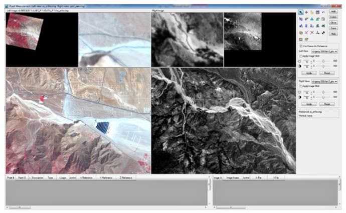
In the Point Measurement tool, click the checkbox next to Use Viewer As Reference (G). The Point Measurement tool automatically changes to display the reference image xs_ortho, in the left view of the point measurement tool, and the original image, spot_pan, in the right view. This can be seen below in Figure 8.

Figure 8: This is a screenshot of the two views that contain the images used in this part of the lab. The xs_ortho.img is on the left and the spot_pan.img is on the right.
Image created by: Cyril Wilson

You will collect reference coordinates by selecting points in xs_ortho, the reference image that correspond to points in the block image, spot_pan. The following is the process of collecting these GCPs with helpful images.

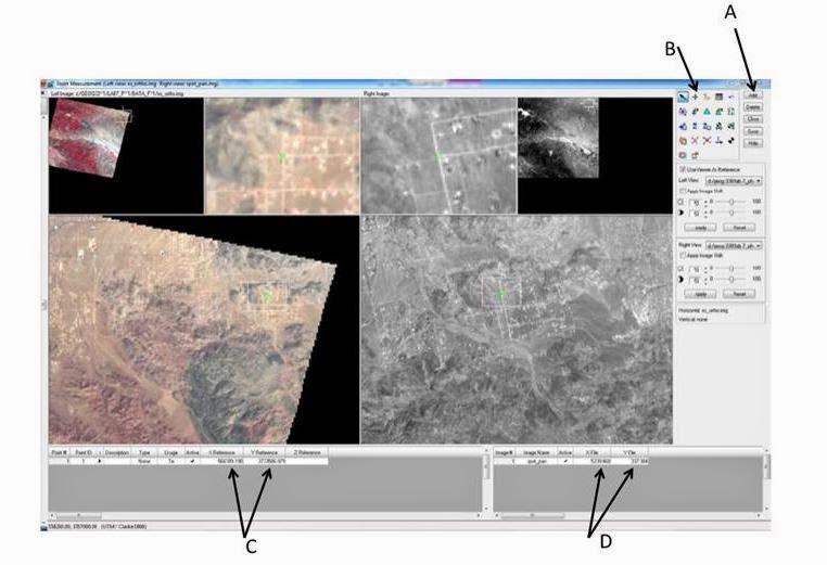
Move the inquire box in the top left viewer showing the full extent of the xs_ortho image to where point ID 1 is (Shown in the Figure below). Click the Add button (A) in the Point Measurement tool. A row for Point ID 1 is added to the reference Cell Array. Move the inquire box in the lower left viewer containing the second view of the xs_ortho image, the detailed view also moves. Do this until you find the road intersectionin the detailed view, shown below.

Figure 9: This is a screenshot for the completion of the directions that are listed for this section.
Image created by: Cyril Wilson

Click the Create Point icon (B). Go to the Detail view on the xs_ortho image and click the road intersection, shown in green. Paint ID 1 is added to all three viewers containing the xs_ortho image. Check the reference control point coordinated; they should almost match those in the table below.

If the coordinates do not approximate (within 10 meters) of those listed in the table above, type in the correct coordinates from the table in the reference cell array, then press enter on the keyboard.

You will now collect the corresponding point on the block image, spot_pan.img. Check figure 1 for the location of Point ID 1 on the spot_pan image display in the right view of the point measurement tool. Move the inquire box in the views containing the spot_pan image until you see the road intersection. Click the Create Point icon and then click on the intersection. Check your spot_pan control point coordinates; they should approximate those in the table below.

 

 

 If your coordinates do not approximate (within two pixels) those listed in the table above, then type in the correct coordinates in the file cell array, then press enter in your keyboard.

 

This process will be the same process that will be followed for GCPs 2-9. The last two control points, Point ID 11 and Point ID 12 will be collected from a different horizontal reference source than the previous one. For the last two GCPs, you will use NAAP_2m-ortho.img. This is an orthoimage at a scale of 1:40,000 with a spatial resolution of 2 meters.

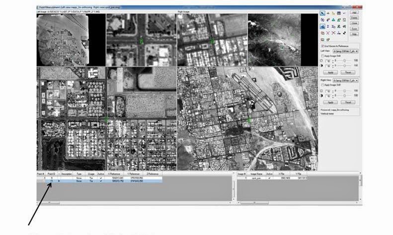
Click the Reset Horizontal Reference Source icon in the Point Measurement tool palette. This opens the GCP Reference Source dialog. Then check the Image Layer radio button. Click OK, opening the Reference Image Layer dialog. Input the image NAAP_2m-ortho.img. Click OK and the NAAP_2m-ortho.img is automatically loaded to the left viewer, shown below in Figure 10. To make the distinction between two different horizontal surfaces (xs_ortho and NAAP_2m-ortho) clearer, skip ID Point 10, and name the next control point Point ID 11.

Figure 10: This is a screenshot of the above process, showing the new images in the left-hand viewer.
Image created by: Cyril Wilson

The process for collecting the ID Points for 11 and 12 will be the same process that was used for points 1-9. When done, click Save and deselect the Use Viewer As Reference checkbox in the Point Measurement tool palette. Now only the spot_pan image will be shown.

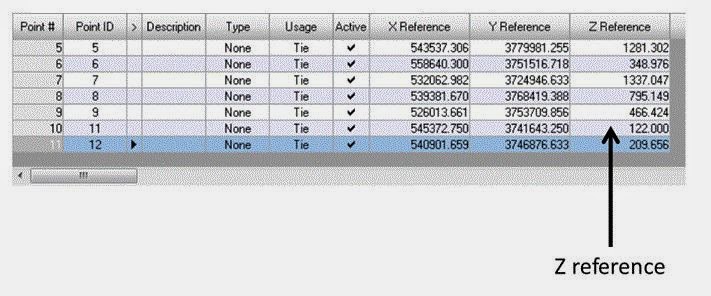
You will not proceed to set the Vertical Reference Source and collect elevation information for all the horizontal reference GCPs you obtained from both images. The image palm_springs_dem.img will be used to collect the elevation information.

In the Point Measurement tool palette, click the Reset Vertical Reference Source icon. The Vertical Reference Source dialog then opens. Click the DEM radio button. Click the dropdown arrow and select Find DEM from the list. In the Add DEM File Name select the DEM palm_springs_dem.img., then click OK in the File Selector.

The DEM file selected displays in the DEM section of the Vertical Reference Source dialog. Click OK. Now right-click on the Point # column and Select All. Click the Update Z Values on Selected Points icon. The Z values of all reference points are updated in the reference cell array based on the values in the DEM selected. This can be seen in Figure 11 below.

Figure 11: This is a screenshot showing the newly acquired Z-values to display elevation for each of the control points.
Image created by: Cyril Wilson

Section 4

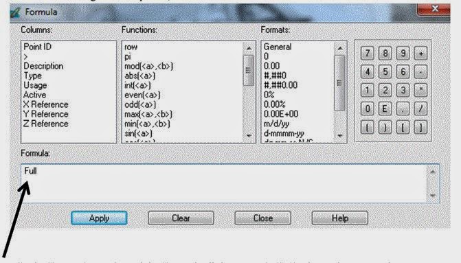
This section deals with set type and usage, with also adding a 2nd image to the block and collecting its GCPs. Left-click the title bar of the column titled Type to select the entire column. Right-click on Type to access the Column Options menu, then select Formula. The Formula dialog is not opened, shown below.

Figure 12: This is a screenshot of the Formula dialog that will be used for this assignment.
Image created by: Cyril Wilson

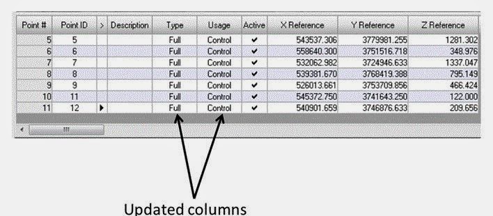
In the Formula section type Full, then click Apply. Each Type entry now changes to indicate Full (X,Y, and Z coordinates). Repeat the above steps to update the Usage column to Control. The cell array should look exactly like the one below.

Figure 13: This is a screenshot that shows the updated columns in the cell array.
Image created by: Cyril Wilson

In the Point Measurement tool, click Save. Then close the Point Management tool, you will be returned to LPS Project Manager.

 

Now that you have successfully finished the collection of reference coordinates from the xs_ortho and NAPP_2m-ortho, and file coordinated in the first block file, spot_pan, you can more on to the second image in the block, spot_panb.img.

 

Click the Add Frame icon and add the image spot_panb.img. Now click Row #2 to highlight the row corresponding to Image ID 2, spot_panb. Click Frame Properties icon. Click OK to accept original perimeters.

 

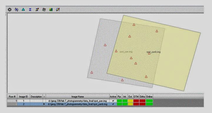
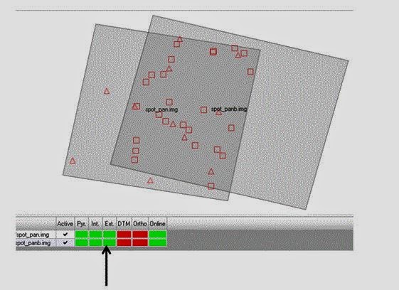
Click the Point measurement icon, select the Classic Point Measurement Tool, and click OK. Spot_panb will be displayed on the left while the initial image in the block spot_pan on the right. Points will be collected for Point ID #1, 2, 6, 8, 9, 12. This is done the exact same way that it was done in section 2. The reason some of the numbers are missing is because they are not located on spot_panb. When you're done click Save. The block interface should look like the image below in Figure 14.

 

 

Figure 14: This is a screenshot of what your Block Interface should look like after completing the steps above.
Image created by: Cyril Wilson

 

 

 

Section 5

 

This section deals with automatic tie points collection, triangulation, and ortho resampling. Begin by clicking the Automatic Tie Point Generation Properties. Image used radio button should be set to All Available. Initial Type radio button should be set to Exterior/Header/GCP. Check and confirm that the Image Layer Used for Computation is set to 1. Click the Distribution tab in the Automatic Tie Point Generation Properties dialog. In the Intended Number of Points/Image field, type in 40. Then click Run. Then click Save and close the Point Measurement tool.

 

 

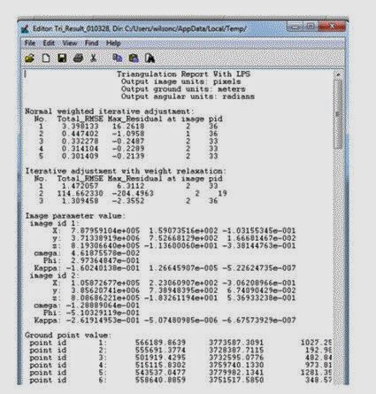
In LPS Project Manager click on Edit-Triangulation Properties. Change the Iterations With Relaxation value to 3. Verify that the Image Coordinate Units for Report is set to Pixels. Click on the Point tab and in the Ground Point Type and Standard Deviations section click the Type dropdown and select Same Weighted Values. Change the values for the X, Y, and Z to 15. Then click Run. This will open a Triangulation Summary report, Figure 15.

 

 

Figure 15: This is a screenshot of what the Triangulation Summary report will look like. This is something that should be looked at and analyzed.
Image created by: Cyril Wilson

 

 

Click Accept and then OK. After returning to the LPS Project Manager click File-Save for the image that is created.

 

 

Figure 16: This is a screenshot of what is produced through completing the above instructions.
Image created by: Cyril Wilson

 

 

Now click the Start Ortho Resampling Process. In the General Tab, click the DTM Source dropdown and select DEM. Click the DEM File Name dropdown and select Find DEM. Input the image palm_springs_dem.img. Click the Output Cell Sizes and change to 10.0. Click the Add button and make sure the second image in the block file spot_panb is in the Input File Name. Check the box to Use Current Cell Sizes, then click OK. Click OK in the Ortho Resampling dialog to start the process. After the model has run click File and Save.

 

 

 

Section 6

 

This last section just deals with viewing the Orthorectified Images. Just bring both the images into the frame and save the results.

 

 

 

Results

 

 

Section 1

 

1.

2 7/8 inches

1 inch = 3,000 ft

2.875” x 3,000’ = 8,625’

8,625’ x 12” = 103,500”

Scale = 1:103,500

2.

Altitude = 20,000 ft.        elevation = 796 ft.            focal length lens = 152 mm. or 0.5 ft.

Scale = f / H – h

Scale = 0.5 / (20,000 – 796)

Scale = (0.5 / 19,204) x 2 =

Scale = 1:38,400

 

Section 2

 

3(a).

37.69 ha, 93.13 acres

3(b).

4175.79 m, 2.59 miles

 

Section 3

 

4.

D = h x r / H

Smoke stack = 0.5 inches              scale = 1:3,209                   H = 3,980 ft.

3,209” x 0.5” = 1,604.5” / 12 = 133.7 ft.

Real world height = 133.7 ft.

Radial distance = 9.5” / 12 = 0.79’

D = (133.7 x 0.79) / 3,980

D = 0.027 x 12 = 0.32 inches

The feature must be plotted inwards 0.32 inches

 

 

Section 4

 

5.

From observing the anaglyph, it is apparent that there are massive flood plains that stretch landward from the river. The elevation for these land areas is fairly similar to that of the river. The area of lower campus is located on that flood plain, and is the student housing area. The student housing area, by Water Street, has a more decreasing elevation as it reaches the river than that of the lower campus area. The difference between the elevations of upper and lower campus are very apparent. The area where Carson Park is located, being surrounded by Half Moon Lake, is at a higher elevation than I would have expected. It is more elevated than both of the previous areas that were talked about. The land located near the southern part of the river in this image is at an extremely low elevation, almost matching that of the river itself.

6.

I believe what I have described is very accurate to that of reality. I’m not really sure about the southern portion of the river, but I do know that the area of land located near the river on the student housing side near Water Street experiences flooding every year in the spring. The sidewalks are closed off because of this flooding. This is explained by the intense decrease in elevation as you get closer to the river. There are some differences, but they aren’t very noticeable because of the lack of flooding in this part of the state.

7.

Like I said in the paragraph prior, this portion of the state doesn’t exactly see much flooding. So in the anaglyph, it might show lower elevations near the river that represent an outwash plain. But in reality we never get that much flooding, so these elevations patterns can be seen as a misconception. In the anaglyph you may think an area would receive a lot of flooding because of the low elevation, but because of the portion of the state we live in this is untrue.

It’s amazing how in the original city image of Eau Claire the elevation differences are almost non-apparent, whereas the anaglyph image the elevation differences jump off the page at you, literally.

 

 

Section 6

 

8.

I’m actually astounded at the accuracy of the spatial overlap between these two images. I zoomed way in to the overlap area and there is seemingly no difference; roads and rivers connect perfectly from one image to another. When you zoom way in the obvious overlap of pixels is apparent, but at a further distance out the overlap is unnoticeable. When you Fit To Frame the overlap area is featured as a black line though, and when you are zoomed in there is a slight difference in shading between the two images. But everything matches up otherwise.

 

 

Geometric Correction

Lab 6

 

 

 

Introduction

 

This week in lab we focused on the idea of Geometric Correction. Geometric correction is the removal of geometric distortion in an imagery so that individual pixels can be in their proper planimetric (x,y) position. This lab was structured to develop your skills on the two major types of geometric correction that are normally performed on satellite images as part of the preprocessing activities prior to the extraction of biophysical and sociocultural information from satellite images.

 

 

 

Methods

 

 

Part 1

 

First open up ERDAS Imagine with a viewer. In this viewer bring in the image Chicago_drg.img. Then open a second viewer and bring in the image Chicago_2000.img. Click Multispectral and then on Control Points. This process can be seen below in Figure 1.

 

 

Figure 1: This is a screenshot of the process of selecting the Control Points tab.
Image created by: Cyril Wilson

 

 

 

Now the Set Geometric Model window will be open, under Select Geometric Model select Polynomial and then hit Ok. Another window will pop up, accept the default. Then navigate to the Lab 6 folder and add your reference DRG image - Chicago_drg.img. Then click Ok on the Reference Map Information.

 

The Multipoint Geometric Correction window will open up two panes. On the left is the input image (Chicago_2000.img), while the reference image is on the right pane (Chicago_drg.img). Each of these panes contains three windows. The top left and top right panes show the entire input and reference images respectively. The other two central top panes shows the areas that are zoomed into on the input image and also that zoomed into the reference image.

 

Now starts the process of adding GCPs to the images. But first the default GCPs need to be deleted. Once this is done the task is to add four pairs of GCPs on the images. Even though only three are needed, extra can't hurt and will give a better fit.

 

Begin by clicking on the Create GCP tool at the top of the page. Then add the four GCP points in the locations exactly like shown in Figure 2.

 

 

Figure 2: This is a screenshot of the instructed areas as to where we were supposed to place our sets of GCP points.
Image created by: Cyril Wilson

 

 

Now is the process of making sure you're doing a good job by evaluating your GCPs. This is done by looking at the Root Mean Square (RMS) error. This is shown at the bottom of the page. For this lab the goal is to reach a RMS of below 2.0. This is done by repositioning the GCPs in their correct placed on both images. After all of the RMS values are below 2.0 now comes the process of creating the corrected image begins.

 

 

Begin this process by clicking on the Display Resample Image Dialog. Name the output file Chicago_2000gcr.img and place it into your Lab 6 folder. click ok and then bring the resampled image into your ERDAS viewer.

 

 

 

Part 2

 

This section is essential going to be the same as the first part, with a few changes. The image that will be located in the first viewer will be sierra_leone_east1991.img and Sierra_Leone_east1991grf.img in the second viewer. Click on Multispectral and Control Points again. Click on Polynomial under Select Geometric Model, then click Ok. Set your reference image as Sierra_Leone_east1991grf.img, and click Ok. On Polynomial Model Properties change the polynomial order to 3 and click close.

 

Now begins the process of adding the GCPs again, but this time 12 are going to be added, even though only ten are needed. The GCPs will be located in the exact same location as of those seem in Figure 3.

 

 

 

Figure 3: This is a screenshot of where the GCPs should be located for this section of the lab.
Image created by: Cyril Wilson

 

 

Next click on the Display Resample Image Dialog on the Multipoint Geometric Correction toolbar. Name the output file sl_east_gcc.img. Change the resampling method to bilinear interpolation and click Ok. Now bring the resampled image into the ERDAS viewer.

 

 

 

Results

 

For the results for each section I either can to upload an image or answer a question or two. I will show you my created images and answered questions for each section below.

 

 

Part 1

 

 

 

 

 

 

 

Q1: The Chicago_drg.img image was the image used in an image-to-map rectification. The image data pixel coordinates were rectified/transformed using the map coordinate counterparts. The rectification process involves converting a data file coordinate to some other grid and coordinate system known as a reference system. So this particular image was used as a reference to transform the map.

Q2: The resampling method used above is called spatial interpolation. Spatial interpolation is the use of GCP pairs to establish a geometric coordinate transformation that is applied to rectify the location of pixels in the output image with a value from a pixel in the unrectified input image.

Q3: GCPs must be dispersed throughout the image to achieve a reliable geometric correction.

Q4: A first-order polynomial equation/model is used to fit a plane to the data. This is the fitting of polynomial equations to the GCP data using least-squares criteria to model the corrections directly in the same image domain.

Q5: The minimum number of GCPs needed for a first order polynomial would be 3.

 

 

Part 2

 

 

Q6: UTM (Zone 29)

Q7: 10 GCPs

Q8: Because in part 1 only 3 GCPs were necessary, in this section 10 GCPs are necessary. Currently there are only 9 GCPs, so it will display Model has no solution

 

 

 

 

 

 

 

 

 

Q9: The new image has a greater geometrical correctness. Even though there is still cloud cover in the image it is still easier to identify features on the new image. The old image was much more distorted and had a lot more cloud cover.

Q10: Bilinear interpolation is more spatially accurate than nearest neighbor. This image was in more need of greater spatial accuracy than the image in part one, that is why bilinear was used instead of nearest neighbor.